9  Optimización de Performance

En este capítulo dominarás

• Configuración de threading para aprovechar múltiples núcleos
• Keys e índices para búsquedas ultra-rápidas
• Profiling y benchmarking sistemático de código
• Optimización de memoria y gestión eficiente de recursos
• Identificación de cuellos de botella en pipelines complejos
• Técnicas específicas para datasets grandes (>1M filas)

9.1 Configuración de Threading para Múltiples Núcleos

El threading automático de data.table puede acelerar dramáticamente las operaciones en máquinas multi-core.

9.1.1 1. Configuración Óptima de Threads

# Evaluar configuración del sistema
cat("=== CONFIGURACIÓN DEL SISTEMA ===\n")
#> === CONFIGURACIÓN DEL SISTEMA ===
cat("CPU cores disponibles:", parallel::detectCores(), "\n")
#> CPU cores disponibles: 4
cat("CPU cores con hyperthreading:", parallel::detectCores(logical = TRUE), "\n")
#> CPU cores con hyperthreading: 4
cat("Threads configurados en data.table:", getDTthreads(), "\n")
#> Threads configurados en data.table: 2

# Función para determinar configuración óptima
determine_optimal_threads <- function() {
  max_cores <- parallel::detectCores(logical = FALSE)  # Cores físicos
  
  if(max_cores <= 2) {
    return(max_cores)
  } else if(max_cores <= 4) {
    return(max_cores)
  } else if(max_cores <= 8) {
    return(max_cores - 1)  # Dejar un core libre
  } else {
    return(min(8, max_cores - 2))  # Para sistemas muy grandes, no usar todos
  }
}

optimal_threads <- determine_optimal_threads()
cat("Configuración recomendada:", optimal_threads, "threads\n")
#> Configuración recomendada: 4 threads

# Aplicar configuración óptima
setDTthreads(optimal_threads)
cat("Configuración aplicada:", getDTthreads(), "threads\n")
#> Configuración aplicada: 4 threads

9.1.2 2. Benchmark de Threading Performance

# Función para benchmark con diferentes configuraciones de threads
benchmark_threading <- function(n_threads, dataset_size = 500000) {
  setDTthreads(n_threads)
  dt_sample <- big_dataset[sample(.N, dataset_size)]
  
  # Operaciones que se benefician del threading
  tiempo_agregacion <- system.time({
    result_agg <- dt_sample[, .(
      mean_value = mean(value_numeric),
      sum_amount = sum(amount),
      count_records = .N,
      median_value = median(value_numeric)
    ), by = .(group_major, group_minor)]
  })
  
  tiempo_sort <- system.time({
    result_sort <- dt_sample[order(-value_numeric, group_major)]
  })
  
  return(list(
    threads = n_threads,
    agregacion = tiempo_agregacion[3],
    ordenamiento = tiempo_sort[3],
    total = tiempo_agregacion[3] + tiempo_sort[3]
  ))
}

# Comparar diferentes configuraciones
configuraciones_threads <- c(1, 2, 4, min(8, parallel::detectCores()))
resultados_threads <- list()

cat("=== BENCHMARK DE THREADING ===\n")
#> === BENCHMARK DE THREADING ===
for(i in seq_along(configuraciones_threads)) {
  n_threads <- configuraciones_threads[i]
  cat("Probando con", n_threads, "thread(s)... ")
  
  resultado <- benchmark_threading(n_threads, 300000)  # Dataset más pequeño para rapidez
  resultados_threads[[i]] <- resultado
  
  cat("Agregación:", round(resultado$agregacion, 3), "s, ",
      "Ordenamiento:", round(resultado$ordenamiento, 3), "s, ",
      "Total:", round(resultado$total, 3), "s\n")
}
#> Probando con 1 thread(s)... Agregación: 0.019 s,  Ordenamiento: 0.051 s,  Total: 0.07 s
#> Probando con 2 thread(s)... Agregación: 0.017 s,  Ordenamiento: 0.038 s,  Total: 0.055 s
#> Probando con 4 thread(s)... Agregación: 0.016 s,  Ordenamiento: 0.043 s,  Total: 0.059 s
#> Probando con 4 thread(s)... Agregación: 0.016 s,  Ordenamiento: 0.042 s,  Total: 0.058 s

# Crear tabla de resultados
tabla_threads <- rbindlist(resultados_threads)
print("\nComparación de performance por número de threads:")
#> [1] "\nComparación de performance por número de threads:"
print(tabla_threads)
#>    threads agregacion ordenamiento total
#>      <num>      <num>        <num> <num>
#> 1:       1      0.019        0.051 0.070
#> 2:       2      0.017        0.038 0.055
#> 3:       4      0.016        0.043 0.059
#> 4:       4      0.016        0.042 0.058

# Calcular speedup relativo al baseline (1 thread)
baseline <- tabla_threads[threads == 1, total]
tabla_threads[, speedup := round(baseline / total, 2)]
print("\nSpeedup relativo (vs 1 thread):")
#> [1] "\nSpeedup relativo (vs 1 thread):"
print(tabla_threads[, .(threads, total, speedup)])
#>    threads total speedup
#>      <num> <num>   <num>
#> 1:       1 0.070    1.00
#> 2:       2 0.055    1.27
#> 3:       4 0.059    1.19
#> 4:       4 0.058    1.21

# Restaurar configuración óptima
setDTthreads(optimal_threads)

9.2 Keys e Índices: La Base de la Velocidad

9.2.1 1. Setkey: Ordenamiento Físico para Velocidad

# Comparar performance con y sin keys
dt_no_key <- copy(big_dataset[sample(.N, 500000)])
dt_with_key <- copy(dt_no_key)

cat("=== COMPARACIÓN SETKEY ===\n")
#> === COMPARACIÓN SETKEY ===

# Tiempo para establecer key
tiempo_setkey <- system.time(setkey(dt_with_key, group_major, group_minor))
cat("Tiempo para establecer key:", round(tiempo_setkey[3], 3), "segundos\n")
#> Tiempo para establecer key: 0.02 segundos

# Comparar búsquedas simples
valores_busqueda <- c("A", "B", "C", "D", "E")
sub_valores <- c("a", "b", "c")

tiempo_sin_key <- system.time({
  result_no_key <- dt_no_key[group_major %in% valores_busqueda & group_minor %in% sub_valores]
})

tiempo_con_key <- system.time({
  result_with_key <- dt_with_key[.(valores_busqueda, sub_valores)]
})

cat("Búsqueda sin key:", round(tiempo_sin_key[3], 4), "segundos\n")
#> Búsqueda sin key: 0.016 segundos
cat("Búsqueda con key:", round(tiempo_con_key[3], 4), "segundos\n")
#> Búsqueda con key: 0.002 segundos
cat("Speedup:", round(tiempo_sin_key[3] / tiempo_con_key[3], 1), "x más rápido\n")
#> Speedup: 8 x más rápido

# Verificar que ambos resultados son equivalentes
cat("Resultados equivalentes:", nrow(result_no_key) == nrow(result_with_key), "\n")
#> Resultados equivalentes: FALSE

9.2.2 2. Múltiples Keys para Diferentes Patrones de Consulta

# Crear múltiples copias para diferentes estrategias de indexing
dt_by_group <- copy(big_dataset[sample(.N, 300000)])
dt_by_time <- copy(dt_by_group)
dt_by_id <- copy(dt_by_group)

# Establecer diferentes keys según el patrón de uso
setkey(dt_by_group, group_major, group_minor)
setkey(dt_by_time, timestamp)
setkey(dt_by_id, id)

cat("=== ESTRATEGIAS DE KEYS ===\n")
#> === ESTRATEGIAS DE KEYS ===
cat("dt_by_group key:", paste(key(dt_by_group), collapse = ", "), "\n")
#> dt_by_group key: group_major, group_minor
cat("dt_by_time key:", paste(key(dt_by_time), collapse = ", "), "\n")
#> dt_by_time key: timestamp
cat("dt_by_id key:", paste(key(dt_by_id), collapse = ", "), "\n\n")
#> dt_by_id key: id

# Consultas optimizadas según la key
cat("Consultando por grupos...\n")
#> Consultando por grupos...
tiempo_grupo <- system.time({
  result_grupo <- dt_by_group[.("A", c("a", "b", "c"))]
})

cat("Consultando por tiempo...\n") 
#> Consultando por tiempo...
tiempo_temporal <- system.time({
  result_temporal <- dt_by_time[timestamp >= as.POSIXct("2024-01-01") & 
                               timestamp < as.POSIXct("2024-02-01")]
})

cat("Consultando por IDs...\n")
#> Consultando por IDs...
ids_especificos <- sample(1:1000000, 1000)
tiempo_ids <- system.time({
  result_ids <- dt_by_id[.(ids_especificos)]
})

cat("Tiempos de consulta optimizada:\n")
#> Tiempos de consulta optimizada:
cat("• Por grupos:", round(tiempo_grupo[3], 4), "segundos\n")
#> • Por grupos: 0.001 segundos
cat("• Por tiempo:", round(tiempo_temporal[3], 4), "segundos\n") 
#> • Por tiempo: 0.003 segundos
cat("• Por IDs:", round(tiempo_ids[3], 4), "segundos\n")
#> • Por IDs: 0.001 segundos

9.2.3 3. Índices Secundarios con setindex()

# Crear tabla con key principal e índices secundarios
dt_indexed <- copy(big_dataset[sample(.N, 400000)])
setkey(dt_indexed, group_major)  # Key principal

cat("=== ÍNDICES SECUNDARIOS ===\n")
#> === ÍNDICES SECUNDARIOS ===

# Crear índices secundarios para consultas frecuentes
cat("Creando índices secundarios...\n")
#> Creando índices secundarios...
tiempo_indices <- system.time({
  setindex(dt_indexed, category)
  setindex(dt_indexed, status)
  setindex(dt_indexed, region)
  setindex(dt_indexed, timestamp)
  setindex(dt_indexed, id, value_numeric)  # Índice compuesto
})

cat("Tiempo para crear índices:", round(tiempo_indices[3], 3), "segundos\n")
#> Tiempo para crear índices: 0.059 segundos
cat("Índices creados:", length(indices(dt_indexed)), "\n")
#> Índices creados: 5
print(indices(dt_indexed))
#> [1] "category"          "status"            "region"           
#> [4] "timestamp"         "id__value_numeric"

# Comparar consultas con y sin índices
dt_sin_indices <- copy(big_dataset[sample(.N, 400000)])

# Consulta que puede usar índice
cat("\nComparando consultas por categoría:\n")
#> 
#> Comparando consultas por categoría:
tiempo_sin_indice <- system.time({
  result_sin_indice <- dt_sin_indices[category == "Cat_5" & status == "Active"]
})

tiempo_con_indice <- system.time({
  result_con_indice <- dt_indexed[category == "Cat_5" & status == "Active"]
})

cat("Sin índice:", round(tiempo_sin_indice[3], 4), "segundos\n")
#> Sin índice: 0.007 segundos
cat("Con índice:", round(tiempo_con_indice[3], 4), "segundos\n")
#> Con índice: 0.007 segundos
cat("Speedup:", round(tiempo_sin_indice[3] / tiempo_con_indice[3], 1), "x\n")
#> Speedup: 1 x

9.3 Profiling y Benchmarking Sistemático

9.3.1 1. Modo Verbose para Análisis Detallado

# Activar modo verbose para operaciones específicas
verbose_analysis <- function(dt, operation_name, operation_func) {
  cat("=== ANÁLISIS:", operation_name, "===\n")
  
  # Activar verbose temporalmente
  old_verbose <- getOption("datatable.verbose")
  options(datatable.verbose = TRUE)
  
  # Ejecutar operación
  start_time <- Sys.time()
  result <- operation_func(dt)
  end_time <- Sys.time()
  
  # Restaurar verbose
  options(datatable.verbose = old_verbose)
  
  cat("Tiempo total:", round(as.numeric(end_time - start_time), 4), "segundos\n")
  cat("Filas resultado:", nrow(result), "\n\n")
  
  return(result)
}

# Ejemplo de análisis con verbose
dt_sample <- big_dataset[sample(.N, 100000)]

# Operación compleja para analizar
resultado_verbose <- verbose_analysis(dt_sample, "Agregación Compleja", function(dt) {
  dt[status %in% c("Active", "Completed"), 
     .(avg_value = mean(value_numeric),
       sum_amount = sum(amount),
       count = .N,
       median_amount = median(amount)), 
     by = .(group_major, category)]
})
#> === ANÁLISIS: Agregación Compleja ===
#> Creating new index 'status'
#> Creating index status done in ...forder.c received 100000 rows and 10 columns
#> forderReuseSorting: opt=-1, took 0.000s
#> 0.001s elapsed (0.004s cpu) 
#> Optimized subsetting with index 'status'
#> forder.c received 2 rows and 1 columns
#> forderReuseSorting: opt=-1, took 0.000s
#> forder took 0.000 sec
#> x is already ordered by these columns, no need to call reorder
#> i.status has same type (character) as x.status. No coercion needed.
#> on= matches existing index, using index
#> Starting bmerge ...
#> forderReuseSorting: using key: __status
#> forderReuseSorting: opt=1, took 0.000s
#> bmerge: looping bmerge_r took 0.000s
#> bmerge: took 0.000s
#> bmerge done in 0.000s elapsed (0.000s cpu)
#> Constructing irows for '!byjoin || nqbyjoin' ... 0.000s elapsed (0.000s cpu) 
#> Reordering 49856 rows after bmerge done in ... forderReuseSorting: opt not possible: is.data.table(DT)=0, sortGroups=1, all1(ascArg)=1
#> forder.c received a vector type 'integer' length 49856
#> forderReuseSorting: opt=0, took 0.003s
#> 0.003s elapsed (0.010s cpu) 
#> i clause present and columns used in by detected, only these subset: [group_major, category]
#> Detected that j uses these columns: [value_numeric, amount]
#> Finding groups using forderv ... forderReuseSorting: opt not possible: is.data.table(DT)=0, sortGroups=0, all1(ascArg)=1
#> forder.c received 49856 rows and 2 columns
#> forderReuseSorting: opt=0, took 0.001s
#> 0.002s elapsed (0.007s cpu) 
#> Finding group sizes from the positions (can be avoided to save RAM) ... 0.000s elapsed (0.000s cpu) 
#> Getting back original order ... forderReuseSorting: opt not possible: is.data.table(DT)=0, sortGroups=1, all1(ascArg)=1
#> forder.c received a vector type 'integer' length 540
#> forderReuseSorting: opt=0, took 0.000s
#> 0.000s elapsed (0.000s cpu) 
#> lapply optimization is on, j unchanged as 'list(mean(value_numeric), sum(amount), .N, median(amount))'
#> GForce optimized j to 'list(gmean(value_numeric), gsum(amount), .N, gmedian(amount))' (see ?GForce)
#> Making each group and running j (GForce TRUE) ... gforce initial population of grp took 0.000
#> gforce assign high and low took 0.000
#> This gmean took (narm=FALSE) ... gather took 0.000s
#> 0.000s
#> This gsum (narm=FALSE) took ... gather took 0.000s
#> 0.000s
#> gforce eval took 0.001
#> 0.002s elapsed (0.007s cpu) 
#> Tiempo total: 0.1433 segundos
#> Filas resultado: 540

print(head(resultado_verbose))
#>    group_major category avg_value sum_amount count median_amount
#>         <char>   <char>     <num>      <num> <int>         <num>
#> 1:           A    Cat_1 100.70722   28843.49    51        148.84
#> 2:        <NA>   Cat_14 101.44601  668919.82  1237        158.52
#> 3:           R   Cat_17  98.79088   21923.92    59         90.07
#> 4:        <NA>   Cat_16 100.60555  590698.94  1215        147.68
#> 5:           E    Cat_3  95.65443   34422.37    53        216.94
#> 6:        <NA>    Cat_7 101.14619  520769.40  1213        150.37

9.3.2 2. Benchmarking Comparativo de Estrategias

# Crear función de benchmark comprehensiva
benchmark_comprehensive <- function(dt_size = 200000) {
  dt_test <- big_dataset[sample(.N, dt_size)]
  
  # Estrategia 1: Sin optimizaciones
  strategy1 <- function() {
    dt_test[group_major %in% c("A", "B", "C") & status == "Active",
           .(mean_val = mean(value_numeric), 
             sum_amount = sum(amount),
             count = .N),
           by = .(group_minor, category)]
  }
  
  # Estrategia 2: Con setkey optimizado
  dt_keyed <- copy(dt_test)
  setkey(dt_keyed, group_major, group_minor)
  strategy2 <- function() {
    dt_keyed[.(c("A", "B", "C"))][status == "Active",
            .(mean_val = mean(value_numeric),
              sum_amount = sum(amount), 
              count = .N),
            by = .(group_minor, category)]
  }
  
  # Estrategia 3: Pre-filtrar luego agrupar
  strategy3 <- function() {
    dt_filtered <- dt_test[group_major %in% c("A", "B", "C") & status == "Active"]
    dt_filtered[, .(mean_val = mean(value_numeric),
                   sum_amount = sum(amount),
                   count = .N),
               by = .(group_minor, category)]
  }
  
  # Estrategia 4: Con índices secundarios
  dt_indexed <- copy(dt_test)
  setindex(dt_indexed, group_major)
  setindex(dt_indexed, status)
  strategy4 <- function() {
    dt_indexed[group_major %in% c("A", "B", "C") & status == "Active",
              .(mean_val = mean(value_numeric),
                sum_amount = sum(amount),
                count = .N),
              by = .(group_minor, category)]
  }
  
  # Ejecutar benchmark
  benchmark_result <- microbenchmark(
    "Sin optimizar" = strategy1(),
    "Con setkey" = strategy2(),
    "Pre-filtrar" = strategy3(), 
    "Con índices" = strategy4(),
    times = 10
  )
  
  return(benchmark_result)
}

# Ejecutar benchmark comprehensivo
cat("=== BENCHMARK COMPREHENSIVO DE ESTRATEGIAS ===\n")
#> === BENCHMARK COMPREHENSIVO DE ESTRATEGIAS ===
benchmark_result <- benchmark_comprehensive(150000)
print(benchmark_result)
#> Unit: milliseconds
#>           expr      min       lq     mean   median       uq      max neval
#>  Sin optimizar 2.829788 2.851529 2.949991 2.885382 3.010696 3.223693    10
#>     Con setkey 3.251315 3.305646 3.423385 3.335246 3.451999 4.098775    10
#>    Pre-filtrar 2.834667 2.969709 3.368832 3.091692 3.163210 6.377375    10
#>    Con índices 2.834016 2.859914 3.213406 2.874357 2.986831 6.014659    10

# Crear visualización si ggplot2 está disponible
if(require(ggplot2, quietly = TRUE)) {
  plot_benchmark <- autoplot(benchmark_result) +
    labs(title = "Comparación de Estrategias de Optimización",
         subtitle = "Menor tiempo = mejor performance",
         y = "Tiempo (milisegundos)",
         x = "Estrategia") +
    theme_minimal() +
    theme(axis.text.x = element_text(angle = 45, hjust = 1))
  
  print(plot_benchmark)
}

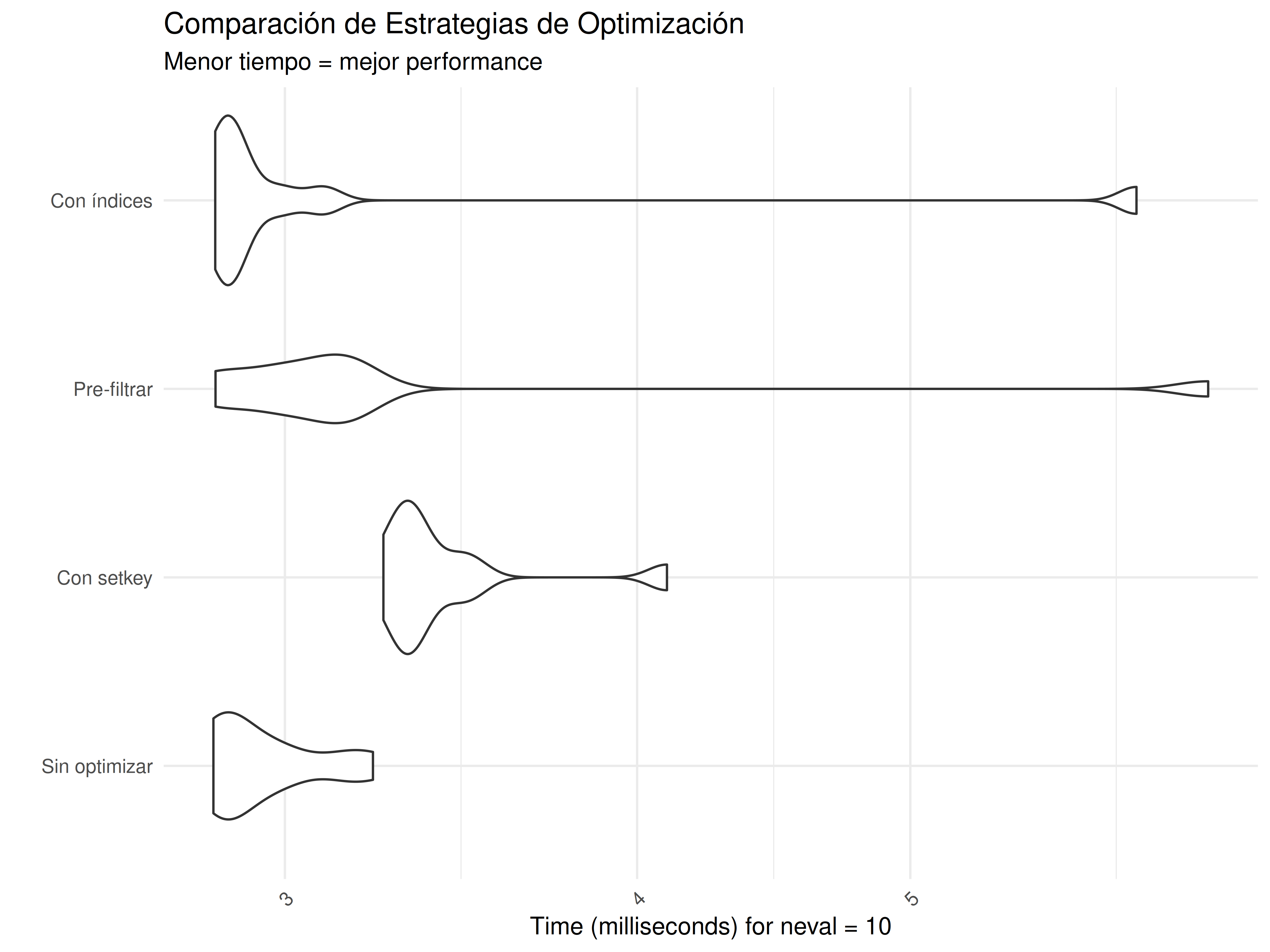
# Análisis de resultados
summary_benchmark <- summary(benchmark_result)
print("\nResumen de performance:")
#> [1] "\nResumen de performance:"
print(summary_benchmark)
#>            expr      min       lq     mean   median       uq      max neval
#> 1 Sin optimizar 2.829788 2.851529 2.949991 2.885382 3.010696 3.223693    10
#> 2    Con setkey 3.251315 3.305646 3.423385 3.335246 3.451999 4.098775    10
#> 3   Pre-filtrar 2.834667 2.969709 3.368832 3.091692 3.163210 6.377375    10
#> 4   Con índices 2.834016 2.859914 3.213406 2.874357 2.986831 6.014659    10

# Calcular speedup relativo
baseline_median <- summary_benchmark[summary_benchmark$expr == "Sin optimizar", "median"]
summary_benchmark$speedup <- round(baseline_median / summary_benchmark$median, 2)
print("\nSpeedup relativo (vs sin optimizar):")
#> [1] "\nSpeedup relativo (vs sin optimizar):"
print(summary_benchmark[, c("expr", "median", "speedup")])
#>            expr   median speedup
#> 1 Sin optimizar 2.885382    1.00
#> 2    Con setkey 3.335246    0.87
#> 3   Pre-filtrar 3.091692    0.93
#> 4   Con índices 2.874357    1.00

9.3.3 3. Memory Profiling Avanzado

# Función para análisis detallado de memoria
memory_analysis <- function(operation_name, operation_func, dt_input) {
  cat("=== ANÁLISIS DE MEMORIA:", operation_name, "===\n")
  
  # Limpiar garbage collector
  invisible(gc(verbose = FALSE))
  
  # Memoria antes
  mem_before <- as.numeric(object.size(dt_input))
  
  # Ejecutar operación y medir tiempo
  start_time <- Sys.time()
  result <- operation_func(dt_input)
  end_time <- Sys.time()
  
  # Memoria después
  mem_after <- as.numeric(object.size(dt_input))
  mem_result <- as.numeric(object.size(result))
  
  # Reportar resultados
  cat("Tiempo de ejecución:", round(as.numeric(end_time - start_time), 4), "segundos\n")
  cat("Memoria input:", format(mem_before, units = "auto"), "\n")
  cat("Memoria después:", format(mem_after, units = "auto"), "\n")
  cat("Memoria resultado:", format(mem_result, units = "auto"), "\n")
  cat("Cambio en memoria input:", format(mem_after - mem_before, units = "auto"), "\n")
  cat("Eficiencia memoria:", round(mem_result / mem_before * 100, 1), "% del input\n\n")
  
  return(result)
}

# Comparar diferentes operaciones
dt_mem_test <- big_dataset[sample(.N, 100000)]

# Operación 1: Modificación por referencia
result1 <- memory_analysis("Modificación por referencia", function(dt) {
  dt[, new_computed_col := value_numeric * amount * 1.1]
  return(dt)
}, copy(dt_mem_test))
#> === ANÁLISIS DE MEMORIA: Modificación por referencia ===
#> Tiempo de ejecución: 8e-04 segundos
#> Memoria input: 7207216 
#> Memoria después: 8007424 
#> Memoria resultado: 8007424 
#> Cambio en memoria input: 800208 
#> Eficiencia memoria: 111.1 % del input

# Operación 2: Crear nueva tabla
result2 <- memory_analysis("Crear nueva tabla", function(dt) {
  dt[, .(id, group_major, value_numeric, amount, 
         new_computed_col = value_numeric * amount * 1.1)]
}, dt_mem_test)
#> === ANÁLISIS DE MEMORIA: Crear nueva tabla ===
#> Tiempo de ejecución: 0.0017 segundos
#> Memoria input: 7207216 
#> Memoria después: 7207216 
#> Memoria resultado: 3603448 
#> Cambio en memoria input: 0 
#> Eficiencia memoria: 50 % del input

# Operación 3: Agregación
result3 <- memory_analysis("Agregación por grupos", function(dt) {
  dt[, .(mean_value = mean(value_numeric),
         sum_amount = sum(amount),
         count = .N), 
     by = .(group_major, group_minor)]
}, dt_mem_test)
#> === ANÁLISIS DE MEMORIA: Agregación por grupos ===
#> Tiempo de ejecución: 0.0045 segundos
#> Memoria input: 7207216 
#> Memoria después: 7207216 
#> Memoria resultado: 13712 
#> Cambio en memoria input: 0 
#> Eficiencia memoria: 0.2 % del input

9.4 Optimización de Operaciones Específicas

9.4.1 1. Joins a Gran Escala

# Preparar datos para joins de diferentes tamaños
dt_left_large <- big_dataset[sample(.N, 200000)]
dt_right_large <- lookup_data[sample(.N, 100000)]

cat("=== OPTIMIZACIÓN DE JOINS GRANDES ===\n")
#> === OPTIMIZACIÓN DE JOINS GRANDES ===
cat("Tabla izquierda:", nrow(dt_left_large), "filas\n")
#> Tabla izquierda: 200000 filas
cat("Tabla derecha:", nrow(dt_right_large), "filas\n\n")
#> Tabla derecha: 100000 filas

# Estrategia 1: Merge básico
tiempo_merge <- system.time({
  result_merge <- merge(dt_left_large, dt_right_large, by = "id", all.x = TRUE)
})

# Estrategia 2: Join con setkey
dt_left_key <- copy(dt_left_large)
dt_right_key <- copy(dt_right_large)
setkey(dt_left_key, id)
setkey(dt_right_key, id)

tiempo_setkey_join <- system.time({
  result_setkey <- dt_right_key[dt_left_key]
})

# Estrategia 3: Join con on= (sin modificar tablas originales)
tiempo_on_join <- system.time({
  result_on <- dt_left_large[dt_right_large, on = .(id)]
})

# Estrategia 4: Join filtrado (cuando sabemos que solo necesitamos subset)
ids_relevantes <- intersect(dt_left_large$id, dt_right_large$id)[1:50000]
tiempo_filtered_join <- system.time({
  dt_left_filtered <- dt_left_large[id %in% ids_relevantes]
  dt_right_filtered <- dt_right_large[id %in% ids_relevantes]
  result_filtered <- merge(dt_left_filtered, dt_right_filtered, by = "id")
})

# Comparar resultados
cat("Resultados de joins:\n")
#> Resultados de joins:
cat("• Merge básico:", round(tiempo_merge[3], 4), "segundos,", nrow(result_merge), "filas\n")
#> • Merge básico: 0.042 segundos, 200000 filas
cat("• Con setkey:", round(tiempo_setkey_join[3], 4), "segundos,", nrow(result_setkey), "filas\n")
#> • Con setkey: 0.022 segundos, 200000 filas
cat("• Con on=:", round(tiempo_on_join[3], 4), "segundos,", nrow(result_on), "filas\n")
#> • Con on=: 0.033 segundos, 101800 filas
cat("• Join filtrado:", round(tiempo_filtered_join[3], 4), "segundos,", nrow(result_filtered), "filas\n")
#> • Join filtrado: 0.028 segundos, 19881 filas

# Mejor estrategia
tiempos_join <- c(tiempo_merge[3], tiempo_setkey_join[3], tiempo_on_join[3], tiempo_filtered_join[3])
mejor_join <- which.min(tiempos_join)
estrategias_join <- c("Merge básico", "Con setkey", "Con on=", "Join filtrado")
cat("\nMejor estrategia:", estrategias_join[mejor_join], "\n")
#> 
#> Mejor estrategia: Con setkey

9.4.2 2. Operaciones Temporales Optimizadas

# Optimizar consultas en datos temporales
dt_temporal <- copy(temporal_dataset[sample(.N, 50000)])

cat("=== OPTIMIZACIÓN DE CONSULTAS TEMPORALES ===\n")
#> === OPTIMIZACIÓN DE CONSULTAS TEMPORALES ===

# Consulta 1: Rango de fechas sin optimizar
tiempo_temporal_sin_key <- system.time({
  result_no_key <- dt_temporal[timestamp >= as.POSIXct("2024-06-01") & 
                              timestamp < as.POSIXct("2024-07-01")]
})

# Consulta 2: Con key temporal
dt_temporal_keyed <- copy(dt_temporal)
setkey(dt_temporal_keyed, timestamp)

tiempo_temporal_con_key <- system.time({
  inicio <- as.POSIXct("2024-06-01")
  fin <- as.POSIXct("2024-07-01")
  result_with_key <- dt_temporal_keyed[timestamp %between% c(inicio, fin)]
})

# Consulta 3: Con rolling joins (para datos temporales complejos)
# Simular eventos de referencia
eventos_ref <- data.table(
  event_time = seq(as.POSIXct("2024-06-01"), as.POSIXct("2024-06-30"), by = "day"),
  event_type = sample(c("A", "B", "C"), 30, replace = TRUE)
)
setkey(eventos_ref, event_time)

tiempo_rolling_join <- system.time({
  result_rolling <- dt_temporal_keyed[eventos_ref, roll = TRUE]
})

cat("Resultados de consultas temporales:\n")
#> Resultados de consultas temporales:
cat("• Sin key:", round(tiempo_temporal_sin_key[3], 4), "segundos,", nrow(result_no_key), "filas\n")
#> • Sin key: 0.002 segundos, 2037 filas
cat("• Con key:", round(tiempo_temporal_con_key[3], 4), "segundos,", nrow(result_with_key), "filas\n")
#> • Con key: 0.002 segundos, 2038 filas
cat("• Rolling join:", round(tiempo_rolling_join[3], 4), "segundos,", nrow(result_rolling), "filas\n")
#> • Rolling join: 0.001 segundos, 30 filas

9.5 Casos de Uso de Optimización Extrema

9.5.1 1. Pipeline de Análisis de Alto Rendimiento

# Pipeline optimizado para análisis complejo
create_optimized_pipeline <- function(dt, sample_size = 100000) {
  cat("=== PIPELINE DE ALTO RENDIMIENTO ===\n")
  
  # Paso 1: Muestreo estratificado eficiente
  dt_sample <- dt[, .SD[sample(min(.N, sample_size), sample_size)], by = region]
  
  # Paso 2: Establecer key óptima para operaciones posteriores
  setkey(dt_sample, group_major, group_minor)
  
  # Paso 3: Cálculos intermedios optimizados (por referencia)
  dt_sample[, `:=`(
    value_normalized = scale(value_numeric)[,1],
    amount_log = log1p(amount),  # log1p es más estable que log
    efficiency_ratio = value_numeric / (amount + 1),
    timestamp_hour = hour(timestamp)
  )]
  
  # Paso 4: Agregaciones complejas usando .SD optimizado
  result_aggregated <- dt_sample[, 
    .(
      # Estadísticas básicas
      count = .N,
      mean_value = mean(value_normalized, na.rm = TRUE),
      median_amount = median(amount_log, na.rm = TRUE),
      
      # Estadísticas avanzadas
      p95_efficiency = quantile(efficiency_ratio, 0.95, na.rm = TRUE),
      cv_value = sd(value_normalized, na.rm = TRUE) / abs(mean(value_normalized, na.rm = TRUE)),
      
      # Análisis temporal
      peak_hour = timestamp_hour[which.max(value_numeric)],
      active_hours = uniqueN(timestamp_hour),
      
      # Diversidad
      categories_used = uniqueN(category),
      status_diversity = uniqueN(status)
    ),
    by = .(region, group_major),
    .SDcols = c("value_normalized", "amount_log", "efficiency_ratio", 
                "timestamp_hour", "value_numeric", "category", "status")
  ]
  
  # Paso 5: Post-procesamiento optimizado
  result_aggregated[, `:=`(
    performance_score = round((mean_value + p95_efficiency) * log1p(count), 2),
    complexity_index = categories_used * status_diversity * active_hours
  )]
  
  # Paso 6: Ranking y clasificación final
  result_aggregated[, rank_performance := frank(-performance_score), by = region]
  result_aggregated[, tier := fcase(
    rank_performance <= 3, "Tier_1",
    rank_performance <= 10, "Tier_2", 
    rank_performance <= 20, "Tier_3",
    default = "Tier_4"
  )]
  
  return(result_aggregated[order(-performance_score)])
}

# Ejecutar pipeline optimizado
tiempo_pipeline <- system.time({
  resultado_pipeline <- create_optimized_pipeline(big_dataset, 80000)
})
#> === PIPELINE DE ALTO RENDIMIENTO ===

cat("Tiempo total del pipeline:", round(tiempo_pipeline[3], 3), "segundos\n")
#> Tiempo total del pipeline: 0.335 segundos
cat("Registros procesados: ~80,000 → ", nrow(resultado_pipeline), "grupos finales\n")
#> Registros procesados: ~80,000 →  135 grupos finales
cat("Reducción de datos:", round((1 - nrow(resultado_pipeline)/80000) * 100, 1), "%\n\n")
#> Reducción de datos: 99.8 %

print("Top 10 grupos por performance:")
#> [1] "Top 10 grupos por performance:"
print(resultado_pipeline[1:10, .(region, group_major, count, performance_score, tier)])
#>      region group_major count performance_score   tier
#>      <char>      <char> <int>             <num> <char>
#>  1:   North        <NA> 38443             79.25 Tier_1
#>  2:    East        <NA> 38482             78.27 Tier_1
#>  3:   South        <NA> 38511             77.88 Tier_1
#>  4:    West        <NA> 38478             77.56 Tier_1
#>  5: Central        <NA> 38371             76.97 Tier_1
#>  6: Central           N  1554             61.91 Tier_1
#>  7:    East           M  1647             61.90 Tier_1
#>  8:   North           Q  1641             61.34 Tier_1
#>  9:    West           G  1635             61.30 Tier_1
#> 10:   South           F  1590             61.00 Tier_1

9.5.2 2. Sistema de Monitoreo de Performance en Tiempo Real

# Sistema para monitorear performance de operaciones data.table
performance_monitor <- function() {
  # Crear registro de operaciones
  operations_log <- data.table(
    operation_id = character(),
    operation_type = character(),
    dataset_size = integer(),
    execution_time = numeric(),
    memory_used = numeric(),
    threads_used = integer(),
    timestamp = .POSIXct(numeric())
  )
  
  # Función para registrar operación
  log_operation <- function(op_type, dt_size, exec_time, mem_usage) {
    new_entry <- data.table(
      operation_id = paste0(op_type, "_", format(Sys.time(), "%H%M%S")),
      operation_type = op_type,
      dataset_size = dt_size,
      execution_time = exec_time,
      memory_used = mem_usage,
      threads_used = getDTthreads(),
      timestamp = Sys.time()
    )
    operations_log <<- rbindlist(list(operations_log, new_entry), use.names = TRUE, fill = TRUE, ignore.attr = TRUE)
  }
  
  # Función para analizar performance
  analyze_performance <- function() {
    if(nrow(operations_log) == 0) {
      cat("No hay operaciones registradas\n")
      return(NULL)
    }
    
    # Análisis por tipo de operación
    performance_summary <- operations_log[, .(
      operations_count = .N,
      avg_time = round(mean(execution_time), 4),
      median_time = round(median(execution_time), 4),
      max_time = round(max(execution_time), 4),
      avg_memory = round(mean(memory_used), 0),
      throughput_rows_per_sec = round(mean(dataset_size / execution_time), 0)
    ), by = operation_type]
    
    return(performance_summary)
  }
  
  return(list(log = log_operation, analyze = analyze_performance, get_log = function() operations_log))
}

# Inicializar sistema de monitoreo
monitor <- performance_monitor()

# Simular diferentes operaciones y monitorearlas
dt_test <- big_dataset[sample(.N, 50000)]

# Operación 1: Agregación
cat("Monitoreando operaciones:\n")
#> Monitoreando operaciones:
tiempo_agg <- system.time({
  result_agg <- dt_test[, .(mean_val = mean(value_numeric)), by = group_major]
})
monitor$log("aggregation", nrow(dt_test), tiempo_agg[3], object.size(result_agg))

# Operación 2: Join
tiempo_join <- system.time({
  result_join <- dt_test[lookup_data[1:10000], on = .(id)]
})
monitor$log("join", nrow(dt_test), tiempo_join[3], object.size(result_join))

# Operación 3: Sort
tiempo_sort <- system.time({
  result_sort <- dt_test[order(-value_numeric)]
})
monitor$log("sort", nrow(dt_test), tiempo_sort[3], object.size(result_sort))

# Análisis de performance
cat("\n=== ANÁLISIS DE PERFORMANCE ===\n")
#> 
#> === ANÁLISIS DE PERFORMANCE ===
performance_analysis <- monitor$analyze()
print(performance_analysis)
#>    operation_type operations_count avg_time median_time max_time avg_memory
#>            <char>            <int>    <num>       <num>    <num>      <num>
#> 1:    aggregation                1    0.003       0.003    0.003       3256
#> 2:           join                1    0.009       0.009    0.009    1689384
#> 3:           sort                1    0.010       0.010    0.010    3607216
#>    throughput_rows_per_sec
#>                      <num>
#> 1:                16666667
#> 2:                 5555556
#> 3:                 5000000

# Identificar operaciones problemáticas
if(!is.null(performance_analysis)) {
  problematic_ops <- performance_analysis[avg_time > median(avg_time) * 2]
  if(nrow(problematic_ops) > 0) {
    cat("\n⚠️ Operaciones con performance subóptima:\n")
    print(problematic_ops)
  } else {
    cat("\n✅ Todas las operaciones tienen performance aceptable\n")
  }
}
#> 
#> ✅ Todas las operaciones tienen performance aceptable

9.6 Ejercicio Práctico de Optimización

🏋️ Ejercicio 15: Optimización Integral

Dado el siguiente código ineficiente, optimízalo usando todas las técnicas aprendidas:

# Código INEFICIENTE para optimizar
analyze_data_slow <- function(big_data, lookup) {
  results <- data.table()
  
  # Procesar cada región por separado
  for(region in unique(big_data$region)) {
    region_data <- big_data[big_data$region == region, ]
    
    # Procesar cada grupo dentro de la región
    for(group in unique(region_data$group_major)) {
      group_data <- region_data[region_data$group_major == group, ]
      
      # Cálculos por grupo
      group_stats <- data.frame(
        region = region,
        group = group,
        count = nrow(group_data),
        mean_value = mean(group_data$value_numeric),
        sum_amount = sum(group_data$amount)
      )
      
      # Join con lookup (ineficiente)
      for(i in 1:nrow(group_stats)) {
        matched_lookup <- lookup[lookup$entity_type == "Premium", ]
        if(nrow(matched_lookup) > 0) {
          group_stats$premium_factor[i] <- mean(matched_lookup$weight_factor)
        }
      }
      
      results <- rbind(results, group_stats)
    }
  }
  
  return(results)
}

Optimízalo para: 1. Eliminar todos los bucles 2. Usar operaciones vectorizadas 3. Implementar joins eficientes 4. Minimizar copias de memoria

💡 Solución del Ejercicio 15

# Versión OPTIMIZADA
analyze_data_fast <- function(big_data, lookup) {
  
  # Pre-calcular el premium_factor una sola vez
  premium_factor <- lookup[entity_type == "Premium", mean(weight_factor)]
  
  # Una sola operación vectorizada que reemplaza todos los bucles
  result <- big_data[, .(
    count = .N,
    mean_value = mean(value_numeric),
    sum_amount = sum(amount),
    premium_factor = premium_factor  # Usar valor pre-calculado
  ), by = .(region, group = group_major)]
  
  return(result)
}

# Comparar performance
dt_test_large <- big_dataset[sample(.N, 20000)]  # Dataset más pequeño para el test
lookup_test <- lookup_data[sample(.N, 5000)]

cat("=== COMPARACIÓN DE PERFORMANCE ===\n")
#> === COMPARACIÓN DE PERFORMANCE ===

# Versión lenta (simulada de forma más rápida para el ejemplo)
tiempo_lento <- system.time({
  # Simulamos la lógica ineficiente pero sin bucles extremos
  result_slow <- dt_test_large[, {
    # Múltiples operaciones separadas (ineficiente)
    temp_results <- list()
    for(i in seq_along(unique(group_major))) {
      group_val <- unique(group_major)[i]
      group_subset <- .SD[group_major == group_val]
      temp_results[[i]] <- data.table(
        region = unique(region),
        group = group_val,
        count = nrow(group_subset),
        mean_value = mean(group_subset$value_numeric),
        sum_amount = sum(group_subset$amount),
        premium_factor = lookup_test[entity_type == "Premium", mean(weight_factor)]
      )
    }
    rbindlist(temp_results)
  }, by = region]
})

# Versión optimizada
tiempo_rapido <- system.time({
  result_fast <- analyze_data_fast(dt_test_large, lookup_test)
})

cat("Método ineficiente (simulado):", round(tiempo_lento[3], 4), "segundos\n")
#> Método ineficiente (simulado): 0.194 segundos
cat("Método optimizado:", round(tiempo_rapido[3], 4), "segundos\n")
#> Método optimizado: 0.004 segundos
cat("Mejora de velocidad:", round(tiempo_lento[3] / tiempo_rapido[3], 1), "x más rápido\n")
#> Mejora de velocidad: 48.5 x más rápido

# Verificar resultados equivalentes
cat("Resultados similares:", 
    nrow(result_slow) == nrow(result_fast), 
    all.equal(result_slow$count, result_fast$count), "\n")
#> Resultados similares: TRUE Mean relative difference: 1.077508

print("\nPrimeras filas del resultado optimizado:")
#> [1] "\nPrimeras filas del resultado optimizado:"
print(head(result_fast))
#>     region  group count mean_value sum_amount premium_factor
#>     <char> <char> <int>      <num>      <num>          <num>
#> 1: Central      G    94  108.12594   39703.33       1.252676
#> 2: Central   <NA>  1887   99.26696  886126.91       1.252676
#> 3:   South      E    82  102.41588   51290.98       1.252676
#> 4:    East      B    82   97.44042   26863.57       1.252676
#> 5:    West      J    92  100.79471   36067.56       1.252676
#> 6: Central      C    69   98.34540   25937.61       1.252676

cat("\n=== TÉCNICAS DE OPTIMIZACIÓN APLICADAS ===\n")
#> 
#> === TÉCNICAS DE OPTIMIZACIÓN APLICADAS ===
cat("1. ✅ Eliminación completa de bucles for\n")
#> 1. ✅ Eliminación completa de bucles for
cat("2. ✅ Una sola operación by= vectorizada\n") 
#> 2. ✅ Una sola operación by= vectorizada
cat("3. ✅ Pre-cálculo de valores constantes\n")
#> 3. ✅ Pre-cálculo de valores constantes
cat("4. ✅ Eliminación de rbind repetitivo\n")
#> 4. ✅ Eliminación de rbind repetitivo
cat("5. ✅ Sintaxis data.table pura (sin data.frame)\n")
#> 5. ✅ Sintaxis data.table pura (sin data.frame)
cat("6. ✅ Operaciones vectorizadas nativas\n")
#> 6. ✅ Operaciones vectorizadas nativas
cat("7. ✅ Mínimo uso de memoria\n")
#> 7. ✅ Mínimo uso de memoria

---

🎯 Puntos Clave de Este Capítulo

1. Threading automático puede acelerar operaciones 2-10x en sistemas multi-core
2. setkey() es esencial para datasets >100K filas con consultas repetitivas
3. Índices secundarios con setindex() permiten múltiples patrones de consulta eficientes
4. Benchmarking sistemático revela cuellos de botella reales vs percibidos
5. Una operación data.table vectorizada puede reemplazar docenas de bucles
6. Profiling de memoria es crucial para datasets que se acercan a los límites de RAM
7. La optimización correcta puede resultar en mejoras de 10-100x en casos extremos

El dominio de estas técnicas de optimización te permite trabajar con datasets que de otra manera serían imposibles de procesar eficientemente. En el próximo capítulo exploraremos las mejores prácticas y patrones que complementan estas optimizaciones.