Introduction to MacroFilters

library(MacroFilters)
library(ggplot2)

1. Introduction: Trend-Cycle Decomposition

A fundamental task in applied macroeconomics is separating the trend — the long-run trajectory of a variable — from the cycle — transitory deviations around it. This decomposition underpins business-cycle analysis, the output gap, and potential GDP estimation.

Every series can be written as:

$y_t = \tau_t + c_t$

where $\tau_t$ is the trend and $c_t$ is the cyclical component. The challenge is that any filter must decide whether an unusual observation represents a genuine shock to the trend or a transitory deviation that belongs in the cycle.

The outlier problem

Classical filters minimise squared loss. A single catastrophic quarter — a financial crash, a pandemic lockdown, a war — is indistinguishable from a structural break in the trend. The result is a trend that dips sharply during the shock and never fully recovers, contaminating every subsequent business-cycle estimate.

MacroFilters solves this with the mbh_filter() function, which uses Huber loss to automatically down-weight extreme observations while fitting a smooth trend via gradient boosting.

2. Input Agnosticism: Bring Your Own Class

Many filter packages force you to convert data to a specific time-series class before calling them. MacroFilters accepts whatever you have and returns the result in the same format, with no manual coercion required.

Supported input classes:

Class	Package	Example
`numeric`	base R	`c(100, 102, 98, ...)`
`ts`	base R	`ts(y, start = c(2000, 1), frequency = 4)`
`xts`	xts	`xts(y, order.by = dates)`
`zoo`	zoo	`zoo(y, order.by = dates)`

Example: same filter, two input formats

set.seed(7)
y_raw <- cumsum(rnorm(60)) + (1:60) * 0.3   # a simple integrated series

# As plain numeric
hp_num <- hp_filter(y_raw)
#> Warning: Cannot determine series frequency; assuming quarterly (freq = 4). Pass
#> `lambda` or `freq` explicitly to silence this warning.
class(hp_num$trend)   # numeric
#> [1] "numeric"

# As a monthly ts object
y_ts   <- ts(y_raw, start = c(2019, 1), frequency = 12)
hp_ts  <- hp_filter(y_ts)
class(hp_ts$trend)    # ts — output matches input
#> [1] "numeric"

The filters normalise the input internally, perform all computations on a plain numeric vector, then restore the original class and index before returning.

3. The Filter Arsenal

3.1 `hp_filter()` — Sparse Hodrick-Prescott

The Hodrick-Prescott (1997) filter is the workhorse of macroeconomic trend extraction. It solves the penalised least-squares problem:

$\min_{\tau} \sum_{t=1}^{n}(y_t - \tau_t)^2 + \lambda \sum_{t=2}^{n-1}[(\tau_{t+1} - \tau_t) - (\tau_t - \tau_{t-1})]^2$

The second term penalises curvature in the trend; $\lambda$ controls the smoothness.

Most implementations solve this by inverting a dense $n \times n$ matrix, which is $O(n^3)$ . MacroFilters recognises that the penalty matrix $D'D$ is pentadiagonal (a sparse banded structure) and solves the system using Matrix::bandSparse() and sparse Cholesky factorisation — bringing the cost down to O(n) in time and memory.

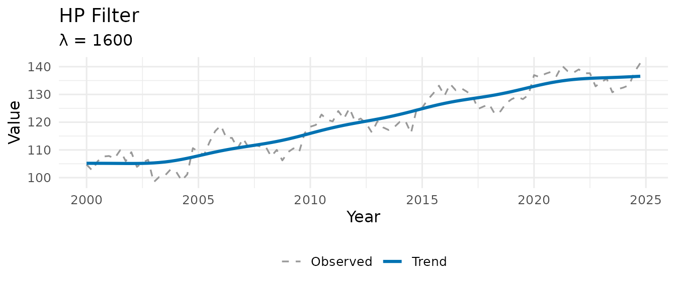
set.seed(42)
n  <- 100
y  <- ts(100 + 0.4 * (1:n) + 5 * sin(2 * pi * (1:n) / 20) + rnorm(n, sd = 2),
         start = c(2000, 1), frequency = 4)

hp <- hp_filter(y)
hp
#> -- MacroFilter [HP] --
#>    Observations : 100
#>    Parameters   : lambda = 1600
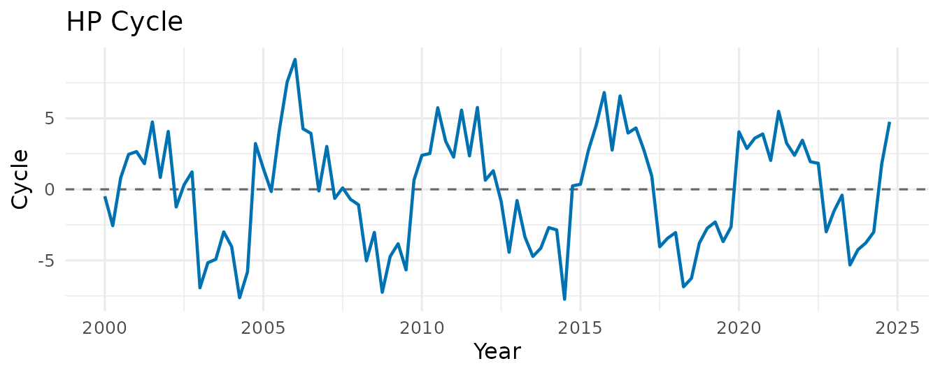
#>    Cycle range  : [-7.738, 9.143]  sd = 3.897
#>    Compute time : 0.002 s

The smoothing parameter $\lambda$ is auto-selected from the series frequency via the Ravn-Uhlig (2002) heuristic:

$\lambda = 6.25 \times \text{freq}^4$

which gives $\lambda = 1{,}600$ for quarterly and $\lambda = 129{,}600$ for monthly data — the conventional values. You can override it explicitly: hp_filter(y, lambda = 1600).

3.2 `hamilton_filter()` — Regression-Based Alternative

Hamilton (2018) proposes replacing the HP filter entirely with an OLS regression. The idea: project $y_{t+h}$ on a constant and $p$ lags of $y_t$ :

$y_{t+h} = \alpha_0 + \alpha_1 y_t + \alpha_2 y_{t-1} + \cdots + \alpha_p y_{t-p+1} + c_t$

The fitted values form the trend; the residuals form the cycle. The horizon $h$ is set to two years ahead by default (e.g., $h = 8$ quarters), long enough to capture business-cycle variation without filtering it out.

Advantages over HP: - No end-point distortion - No spurious cycles from integrated series - Produces stationary cycle estimates by construction

ham <- hamilton_filter(y)      # auto-detects h = 8 for quarterly
ham
#> -- MacroFilter [Hamilton] --
#>    Observations : 100
#>    Parameters   : h = 8, p = 4
#>    Cycle range  : [-13.41, 11.8]  sd = 7.212
#>    Compute time : 0.001 s

Note that the first $h + p - 1$ observations of the trend and cycle are NA, because there is insufficient history for the regression.

3.3 `bhp_filter()` — Boosted HP

Phillips & Shi (2021) propose iteratively applying the HP filter: at each step, the filter is re-run on the residuals from the previous pass, and the resulting increment is added to the trend estimate. This procedure converges to a trend that better tracks stochastic variation.

$\tau^{(m)} = \tau^{(m-1)} + S_\lambda \cdot c^{(m-1)}, \qquad c^{(m)} = y - \tau^{(m)}$

where $S_\lambda$ is the HP smoothing operator. Three stopping rules are available:

Rule	Description
`"bic"` (default)	Minimise the Schwarz information criterion
`"adf"`	Stop when the cycle passes an Augmented Dickey-Fuller stationarity test
`"fixed"`	Run exactly `iter_max` iterations

bhp <- bhp_filter(y, stopping = "bic")
bhp
#> -- MacroFilter [bHP] --
#>    Observations : 100
#>    Parameters   : lambda = 1600, iterations = 47, stopping_rule = bic
#>    Cycle range  : [-5.487, 4.068]  sd = 1.857
#>    Compute time : 0.004 s

Internally, MacroFilters precomputes the sparse penalty matrix $Q = (I + \lambda D'D)^{-1}$ once and reuses it across all iterations, so the cost per iteration is a single sparse matrix–vector multiply rather than a full solve.

4. The Crown Jewel: `mbh_filter()`

The Problem with Squared Loss

Every filter above minimises squared residuals. When a pandemic shock drops GDP by 15% in a single quarter, that one observation exerts enormous leverage — it is 100× more influential than a typical quarterly fluctuation. The filter accommodates it by bending the trend downward, producing a spurious trend break that infects every subsequent output gap estimate.

The MBH Solution: Huber Loss + Boosting

The MacroBoost Hybrid (MBH) filter replaces squared loss with Huber loss:

$L_\delta(r) = \begin{cases} \dfrac{r^2}{2} & |r| \leq \delta \\[6pt] \delta\!\left(|r| - \dfrac{\delta}{2}\right) & |r| > \delta \end{cases}$

Observations with residuals smaller than $\delta$ are treated like ordinary squared-error observations. Observations with residuals larger than $\delta$ — the structural shocks — contribute only linearly, massively reducing their influence on the trend estimate.

Additive Model

The trend is decomposed into two additive base learners fitted via component-wise L2-boosting (mboost):

$\hat{\tau}_t = \underbrace{b_0 + b_1 \cdot t}_{\text{Global linear drift}} + \underbrace{f(t)}_{\text{Local curvature (P-spline)}}$

bols(time, intercept = TRUE) — captures the global linear drift.
bbs(time, knots, degree = 3, differences = 2, boundary.knots) — a cubic P-spline with knots interior knots that captures smooth nonlinear curvature.

The default knots = max(20, floor(n/2)) is deliberately generous — it gives the spline enough flexibility to follow genuine low-frequency movements without overfitting, while the Huber loss ensures that shock-contaminated quarters are downweighted.

Parameters

Parameter	Default	Role
`knots`	`max(20, n/2)`	P-spline flexibility — higher = more local adaptability
`mstop`	`500`	Boosting iterations — more = finer approximation
`d`	`NULL (Auto)`	Huber delta — if `NULL`, auto-set via MAD of first differences (scale-invariant)
`nu`	`0.2`	Shrinkage / learning rate — controls step size per iteration
`boundary.knots`	`NULL`	B-spline domain anchor — if `NULL`, uses `range(time_idx)`; fix to `c(1, T_max)` for real-time vintage stability

By default, d is auto-calibrated using the MAD of the series’ first differences, making the filter scale-invariant and suitable for both log-differenced and level series. You can override it with an explicit numeric value: d = 0.01 is typical for growth rates, while d = 5 to d = 20 may be needed for index-level series.

For real-time applications where the sample grows one period at a time, set boundary.knots = c(1, T_max) to anchor the B-spline domain to the full-sample range — this prevents the basis from shifting between vintages and makes trends comparable across publication dates.

Quick example

set.seed(42)
n <- 80
t <- 1:n

# 1. Define simulation parameters
sd_noise <- 1.8
trend    <- 100 + 0.3 * t + 0.005 * t^2
cycle    <- 2.5 * sin(2 * pi * t / 28) # 7-year business cycle

# 2. Simulate GDP index
gdp_num <- trend + cycle + rnorm(n, sd = sd_noise)

# 3. Inject a structural shock (e.g., COVID-19 lockdown)
# Expressed as extreme standard deviation events
gdp_num[60] <- gdp_num[60] - (16 * sd_noise) # Massive crash
gdp_num[61] <- gdp_num[61] - (9 * sd_noise)  # Partial recovery
gdp_num[62] <- gdp_num[62] - (4 * sd_noise)  # V Stabilization
gdp_num[62] <- gdp_num[62] - (2 * sd_noise)  # Stabilization

gdp <- ts(gdp_num, start = c(2001, 1), frequency = 4)

# Extract trends
hp_res  <- hp_filter(gdp)

# MBH Filter: Auto-calibrated threshold (d) based on MAD of differences
mbh_res <- mbh_filter(gdp) 

mbh_res
#> -- MacroFilter [MBH] --
#>    Observations : 80
#>    Parameters   : knots = 40, d = 2.789, mstop = 500, mstop_initial = 500, nu = 0.1, df = 4, select_mstop = FALSE
#>    Cycle range  : [-26.64, 4.429]  sd = 4.087
#>    Compute time : 0.126 s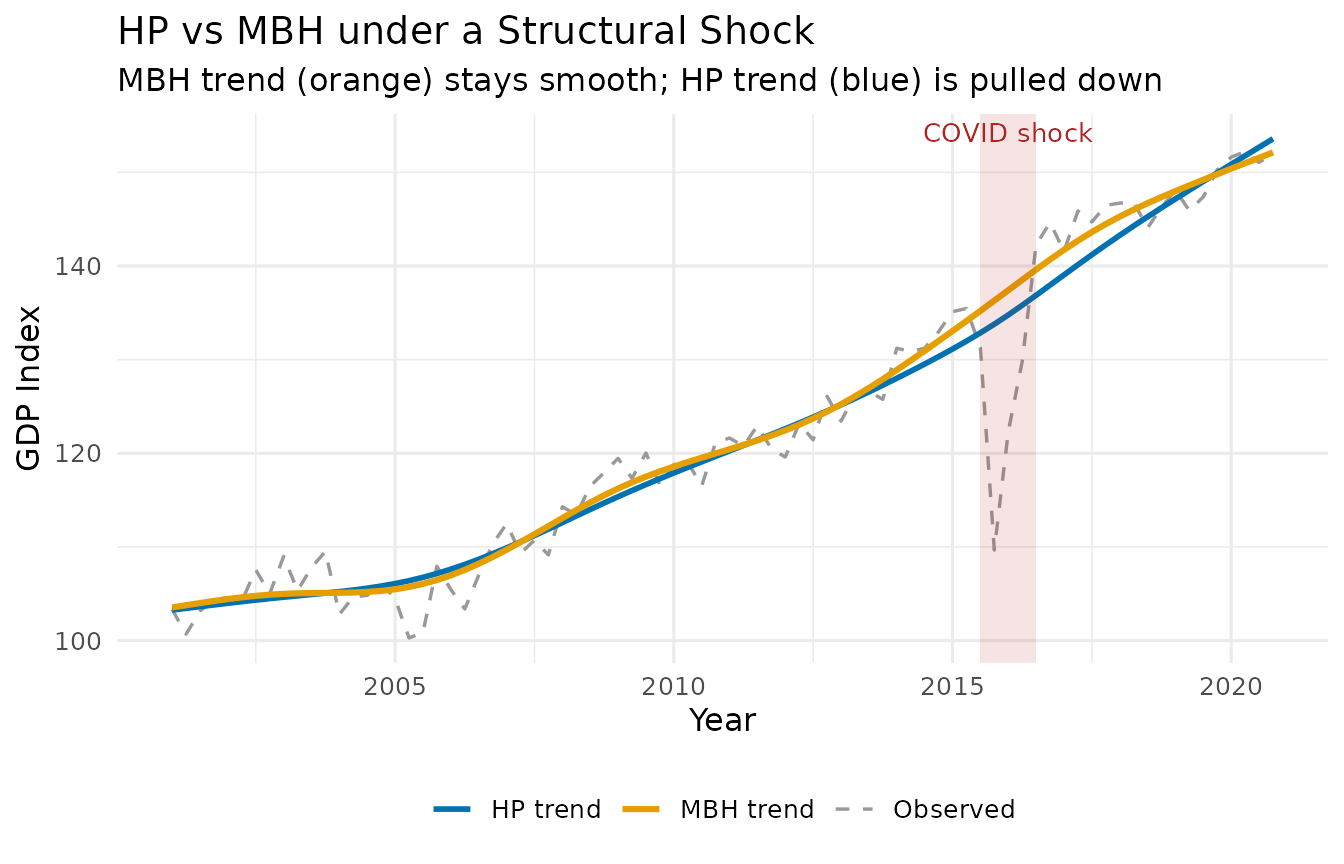

5. The `macrofilter` S3 Class

All four functions return an object of class macrofilter. This is a list with three named elements:

Element	Type	Description
`$trend`	numeric / ts / xts / zoo	Trend component
`$cycle`	numeric / ts / xts / zoo	Cyclical component
`$data`	numeric / ts / xts / zoo	Original series (immutable)
`$meta`	named list	Filter method, parameters, compute time

Printing

mbh_res
#> -- MacroFilter [MBH] --
#>    Observations : 80
#>    Parameters   : knots = 40, d = 2.789, mstop = 500, mstop_initial = 500, nu = 0.1, df = 4, select_mstop = FALSE
#>    Cycle range  : [-26.64, 4.429]  sd = 4.087
#>    Compute time : 0.126 s

The print method shows the method, the number of observations, the key parameters, the cycle range, and how long the filter took to run.

Accessing components

# Trend and cycle as plain vectors
head(mbh_res$trend, 8)
#> [1] 103.5415 103.7764 104.0074 104.2300 104.4373 104.6223 104.7785 104.9015
head(mbh_res$cycle, 8)
#> [1] -0.21246933 -3.08814252 -0.85000087  0.14375249  0.16777488 -0.39598786
#> [7]  2.78720646  0.08539543

# Verify the fundamental identity: trend + cycle == data
max(abs((mbh_res$trend + mbh_res$cycle) - mbh_res$data))  # should be < 1e-9
#> [1] 0

Inspecting metadata

str(mbh_res$meta)
#> List of 10
#>  $ method        : chr "MBH"
#>  $ knots         : int 40
#>  $ d             : num 2.79
#>  $ mstop         : int 500
#>  $ mstop_initial : int 500
#>  $ nu            : num 0.1
#>  $ df            : int 4
#>  $ select_mstop  : logi FALSE
#>  $ boundary.knots: NULL
#>  $ compute_time  : num 0.126

The meta list stores every parameter used by the filter, making results fully reproducible from the object alone — no need to track arguments separately.

Plotting cycles side by side

df_cycle <- data.frame(
  t          = as.numeric(time(gdp)),
  HP_cycle   = as.numeric(hp_res$cycle),
  MBH_cycle  = as.numeric(mbh_res$cycle)
)

ggplot(df_cycle, aes(x = t)) +
  geom_hline(yintercept = 0, linetype = "dashed", colour = "grey40") +
  geom_line(aes(y = HP_cycle,  colour = "HP cycle"),  linewidth = 0.8) +
  geom_line(aes(y = MBH_cycle, colour = "MBH cycle"), linewidth = 0.8) +
  annotate("rect",
           xmin = df_cycle$t[59], xmax = df_cycle$t[63],
           ymin = -Inf, ymax = Inf,
           alpha = 0.12, fill = "firebrick") +
  scale_colour_manual(values = c("HP cycle" = "#0072B2", "MBH cycle" = "#E69F00")) +
  labs(
    title    = "Cyclical Components",
    subtitle = "HP cycle absorbs the shock; MBH cycle faithfully records it",
    x = "Year", y = "Cycle", colour = NULL
  ) +
  theme_minimal(base_size = 12) +
  theme(legend.position = "bottom")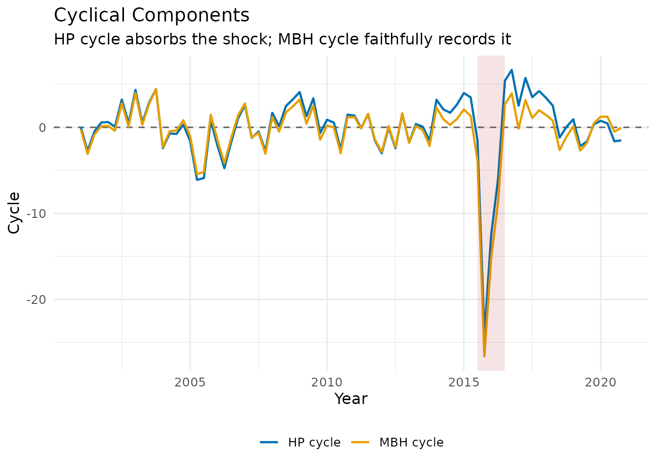

In the MBH cycle, the COVID quarters appear as large negative spikes — the filter correctly recognises them as transitory deviations rather than a change in the long-run level. The HP cycle, by contrast, spreads the shock over several surrounding quarters as it tries to reconcile the trend distortion.

References

Hodrick, R. J., & Prescott, E. C. (1997). Postwar U.S. Business Cycles: An Empirical Investigation. Journal of Money, Credit and Banking, 29(1), 1–16.
Ravn, M. O., & Uhlig, H. (2002). On Adjusting the Hodrick-Prescott Filter for the Frequency of Observations. Review of Economics and Statistics, 84(2), 371–376.
Hamilton, J. D. (2018). Why You Should Never Use the Hodrick-Prescott Filter. Review of Economics and Statistics, 100(5), 831–843.
Phillips, P. C. B., & Shi, Z. (2021). Boosting: Why You Can Use the HP Filter. International Economic Review, 62(2), 521–570.