Hyperparameter Tuning for the MacroBoost Hybrid Filter
Source:vignettes/tuning_mbh.Rmd
tuning_mbh.Rmd1 Anatomy of the MBH Trifecta
mbh_filter() exposes three knobs that jointly govern fit
quality, robustness, and computation time.
| Parameter | Default | Role |
|---|---|---|
mstop |
500 |
Gradient-descent iteration budget |
nu |
0.1 |
Per-step shrinkage (learning rate) |
knots |
min(max(20, floor(n/2)), 250) |
P-spline interior knot count (capped at 250) |
1.1 mstop — iteration budget
Each boosting step adds a small, smooth update to the current trend
estimate. More iterations allow finer approximation of the optimal
solution, at the cost of linear wall time. The default
mstop = 500 is calibrated to produce HP-comparable
flexibility on quarterly macro series (~100–400 observations).
1.2 nu — shrinkage
nu scales the gradient contribution of each step. Lower
nu requires more iterations to reach the same fit quality;
higher nu converges faster but may overshoot. The key
identity is:
A practical equivalence: (mstop = 500, nu = 0.1) and
(mstop = 1000, nu = 0.05) produce nearly identical
trends.
y <- us_gdp_vintage$gdp_log

res_default <- mbh_filter(y, mstop = 500,  nu = 0.10)
#> Info: Huber threshold automatically calibrated to d = 0.004450 via HP cyclical MAD.
res_equiv   <- mbh_filter(y, mstop = 1000, nu = 0.05)
#> Info: Huber threshold automatically calibrated to d = 0.004450 via HP cyclical MAD.

max_diff <- max(abs(res_default$trend - res_equiv$trend))
cat(sprintf("Max trend difference (mstop×nu equivalence): %.2e\n", max_diff))
#> Max trend difference (mstop×nu equivalence): 8.54e-08
1.3 knots — spline flexibility
Knots control how many local basis functions the P-spline uses to
represent the trend shape. The default heuristic
min(max(20, floor(n/2)), 250) provides roughly one knot per
two observations (capped at 250 for long series) — high density relative
to classical smoothing spline recommendations — because Huber loss (not
spline regularity) acts as the primary smoothness constraint.
Too few knots force an overly rigid polynomial-like trend; too many
knots with low mstop may leave some basis functions
unfitted.
2 Auto-calibration of Huber Delta d
The Huber loss function
transitions between (quadratic) loss for small residuals and (absolute) loss for large ones. The threshold determines which residuals are treated as outliers.
When d = NULL, the threshold is set automatically via
the MAD of first differences:
The scale factor makes MAD a consistent estimator of the standard deviation under normality.
2.1 Scale invariance
If , then and . The Huber threshold scales exactly with the data amplitude, so the filter behaves identically regardless of the measurement units.
y_level <- us_gdp_vintage$gdp_real   # billions USD (~20 000 scale)
y_log   <- us_gdp_vintage$gdp_log    # natural log (~10 scale)

d_level <- stats::mad(diff(y_level))
d_log   <- stats::mad(diff(y_log))

cat(sprintf("d (level series) : %.4f\n", d_level))
#> d (level series) : 70.1166
cat(sprintf("d (log series)   : %.6f\n", d_log))
#> d (log series)   : 0.006841
cat(sprintf("Ratio d_level / mean(level): %.6f\n", d_level / mean(y_level)))
#> Ratio d_level / mean(level): 0.006792
cat(sprintf("Ratio d_log   / mean(log)  : %.6f\n", d_log   / mean(y_log)))
#> Ratio d_log   / mean(log)  : 0.000758
2.2 Scale-mismatch warning for log-level input
For log-level GDP, diff(y) returns quarterly growth
rates whose typical scale is 0.004–0.010. The output gap (the cycle the
filter must explain) operates on a much larger scale, typically
0.01–0.05. Using d = mad(diff(y)) therefore sets the Huber
threshold too tight: normal business-cycle oscillations
are mis-classified as outliers, their gradient contributions are
truncated, and the trend becomes a near-straight line.
The recommended override is:
d_cycle <- mad(hp_filter(y_log)$cycle)   # set d on the residual scale
res     <- mbh_filter(y_log, d = d_cycle)
3 Overriding d for High-Volatility Series
Quarterly GDP growth rates (diff(log(GDP))) are roughly
40× more volatile relative to trend than log levels. The COVID collapse
of 2020 Q2
(
q-o-q) represents an extreme outlier even by growth-rate standards. This
makes growth rates an ideal stress test for d
sensitivity.
y_growth <- diff(us_gdp_vintage$gdp_log)   # quarterly log-differences

res_auto   <- mbh_filter(y_growth)
#> Info: Huber threshold automatically calibrated to d = 0.005430 via HP cyclical MAD.
res_strict <- mbh_filter(y_growth, d = 0.005)
res_lenient <- mbh_filter(y_growth, d = 0.02)

cat(sprintf("Auto d = %.6f\n", res_auto$meta$d))
#> Auto d = 0.005430
dt_growth <- data.table(
  t        = us_gdp_vintage$date[-1],
  observed = y_growth,
  auto     = res_auto$trend,
  strict   = res_strict$trend,
  lenient  = res_lenient$trend
)

dt_long <- melt(dt_growth,
                id.vars      = "t",
                measure.vars = c("auto", "strict", "lenient"),
                variable.name = "delta",
                value.name    = "trend")

# Human-readable labels
auto_label <- sprintf("Auto (d=%.4f)", res_auto$meta$d)
# data.table::melt() returns variable.name as factor; fcase() returns character.
# Assigning character to a factor column via := raises a type mismatch error,
# so coerce to character first.
dt_long[, delta := as.character(delta)]
dt_long[, delta := fcase(
  delta == "auto",    auto_label,
  delta == "strict",  "Strict (d=0.005)",
  delta == "lenient", "Lenient (d=0.020)"
)]

colour_vals <- c("#0072B2", "#009E73", "#E69F00")
names(colour_vals) <- c("Strict (d=0.005)", auto_label, "Lenient (d=0.020)")

p_d <- ggplot() +
  geom_line(
    data = dt_growth,
    aes(x = t, y = observed),
    colour = "grey70", linewidth = 0.5
  ) +
  geom_line(
    data = dt_long,
    aes(x = t, y = trend, colour = delta),
    linewidth = 0.9
  ) +
  annotate("rect",
           xmin = as.Date("2020-01-01"), xmax = as.Date("2020-10-01"),
           ymin = -Inf, ymax = Inf, alpha = 0.1, fill = "firebrick") +
  annotate("text", x = as.Date("2020-04-01"), y = Inf,
           label = "COVID Q2\n-9% q-o-q", vjust = 1.4,
           size = 3.2, colour = "firebrick") +
  scale_colour_manual(values = colour_vals) +
  labs(
    title    = "MBH Trend Sensitivity to Huber Delta d",
    subtitle = "Data: US quarterly GDP growth rates (log-diff)",
    x        = NULL, y = "Log-difference", colour = "d setting"
  ) +
  theme_minimal(base_size = 12) +
  theme(legend.position = "top")

print(p_d)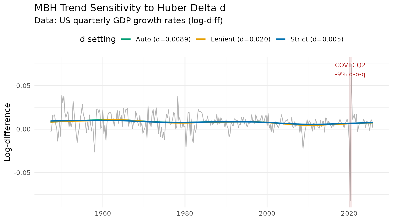
Interpretation
-
Strict
d = 0.005(blue): Huber threshold is tight; even modest growth rate swings are down-weighted. The trend is nearly flat, absorbing almost no cyclical signal. -
Auto
d(green): threshold is calibrated to normal volatility. The COVID spike is substantially down-weighted but ordinary fluctuations are fitted. -
Lenient
d = 0.020(orange): threshold is loose; the filter behaves close to boosting and the trend responds to the COVID shock.
4 Computational Trade-off Benchmark
y          <- us_gdp_vintage$gdp_log
mstop_grid <- seq(100L, 1000L, by = 100L)   # 10 evenly-spaced points
n_rep      <- 5L                            # replicates per point

# Single-shot timings are dominated by GC pauses and OS scheduling, which
# produce spurious spikes. We warm up once, then time several runs with a
# clean heap (gc()) before each and report the MEDIAN, recovering the
# monotone wall-time vs mstop relationship.
bench_dt <- rbindlist(lapply(mstop_grid, function(m) {
  res  <- suppressMessages(mbh_filter(y, mstop = m))   # warm-up + cycle SD
  reps <- vapply(seq_len(n_rep), function(i) {
    gc(verbose = FALSE)
    t0 <- proc.time()
    suppressMessages(mbh_filter(y, mstop = m))
    (proc.time() - t0)[["elapsed"]]
  }, numeric(1))
  data.table(
    mstop       = m,
    elapsed_sec = round(median(reps), 3),
    cycle_sd    = round(sd(res$cycle), 6)
  )
}))

knitr::kable(
  bench_dt,
  col.names = c("mstop", "Wall time (s)", "Cycle SD"),
  caption   = sprintf("MBH computational benchmark — US log GDP (%d obs)", length(y))
)| mstop | Wall time (s) | Cycle SD |
|---|---|---|
| 100 | 0.043 | 0.663846 |
| 200 | 0.067 | 0.625541 |
| 300 | 0.090 | 0.587335 |
| 400 | 0.122 | 0.549249 |
| 500 | 0.139 | 0.511309 |
| 600 | 0.155 | 0.473548 |
| 700 | 0.177 | 0.436016 |
| 800 | 0.193 | 0.398778 |
| 900 | 0.208 | 0.361931 |
| 1000 | 0.223 | 0.325643 |
# Dual-axis layout: wall time (left) + cycle_sd convergence (right)
# Use a secondary-axis trick by normalising cycle_sd to the time scale
time_range  <- range(bench_dt$elapsed_sec)
sd_range    <- range(bench_dt$cycle_sd)
# Guard against division by zero if cycle_sd converges to a flat line
if (diff(sd_range)   < 1e-10) sd_range   <- sd_range   + c(-1e-5,  1e-5)
if (diff(time_range) < 1e-10) time_range <- time_range + c(-1e-5,  1e-5)
sd_to_time  <- function(x) (x - sd_range[1]) / diff(sd_range) * diff(time_range) + time_range[1]
time_to_sd  <- function(x) (x - time_range[1]) / diff(time_range) * diff(sd_range) + sd_range[1]

p_bench <- ggplot(bench_dt, aes(x = mstop)) +
  geom_line(aes(y = elapsed_sec), colour = "#0072B2", linewidth = 1) +
  geom_point(aes(y = elapsed_sec), colour = "#CC0000", size = 3) +
  geom_line(aes(y = sd_to_time(cycle_sd)),
            colour = "#E69F00", linewidth = 0.9, linetype = "dashed") +
  geom_point(aes(y = sd_to_time(cycle_sd)),
             colour = "#E69F00", size = 2.5) +
  scale_x_continuous(breaks = mstop_grid) +
  scale_y_continuous(
    name     = "Wall time (s)  [blue / red points]",
    sec.axis = sec_axis(~ time_to_sd(.), name = "Cycle SD  [orange dashed]",
                        labels = scales::label_number(accuracy = 0.0001))
  ) +
  labs(
    title    = "Wall Time vs Boosting Iterations",
    subtitle = sprintf("US Real GDP log level (%d obs). Cycle SD plateaus well before mstop = 500.", length(y)),
    x        = "mstop"
  ) +
  theme_minimal(base_size = 12) +
  theme(
    axis.title.y.left  = element_text(colour = "#0072B2"),
    axis.title.y.right = element_text(colour = "#E69F00")
  )

print(p_bench)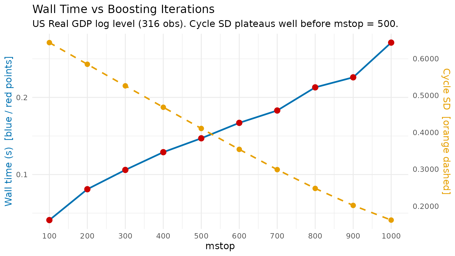
Practical guidance
| Use case | Recommended settings |
|---|---|
| Interactive / exploratory | mstop = 100–200 |
| Publication-quality output |
mstop = 500 (default) |
| Long daily series (n > 5 000) | mstop = 50, nu = 0.3 |
| Cross-country batch estimation | mstop = 200, nu = 0.15 |
Gains in cycle standard deviation (a proxy for fit quality) diminish
rapidly above mstop = 200 for a typical macro series. The
default mstop = 500 provides a comfortable safety margin
without being prohibitively slow.
5 Summary
| Parameter | Default | When to increase | When to decrease |
|---|---|---|---|
mstop |
500 | Publication accuracy required | Exploratory / fast iteration |
nu |
0.1 | Very long series; computational budget tight | Stability preferred over speed |
knots |
min(max(20, n/2), 250) |
Highly nonlinear trend | Short series or near-linear trend |
d |
auto via MAD | Series has frequent large spikes | Series is log-level (use mad(hp$cycle)
instead) |